eNote.Page

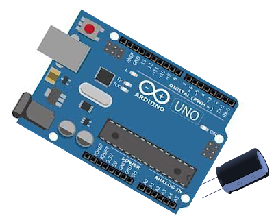
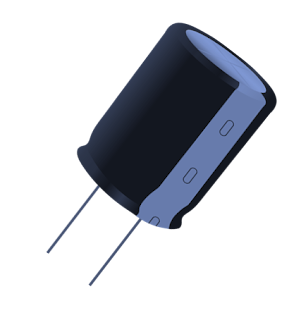
This video tutorial illustrates the Arduino based simulation of capacitance meter / capacitance measurement of capacitors & supercapacitors with Tinkercad simulation.   Principle for this measurement is explained in the following page: https://www.enote.page/2022/01/capacitor-charging-discharging-time.html   Estimation of capacitance of capacitors & supercapacitors by simulating charging & discharging is explained in the following page: https://www.enote.page/2021/06/capacitor-simulation.html   Components required Name Number Component C1 1 100 nF to 10 mF Capacitor R1 1 10 kΩ Resistor U1 1 Arduino Uno R3 board Meter2 1 Voltage meter R2 1 220 Ω Resistor     Increase the resistance value from 10K, if the charging time is too short. Decrease the

This video tutorial explains, how to simulate charging & discharging the capacitors, supercapacitors and ultracapacitors for the estimation of capacitance. This charging-discharging method is used to estimate the capacitance of the capacitors. By simultaneous charging & discharging of a capacitor, its capacitance can be estimated from the time duration and change in potential.   Charging & discharging potential (in Volts) against time (seconds) is recorded under constant resistance (Ohms). If the current is kept constant, it is known as the galvanostatic charging and discharging (GCD) technique. It is used to estimate the specific capacitance of supercapacitors. Charging & discharging potential (in Volts) is plotted against the respective time (in seconds).  From the graph, the capacitance can be estimated. To perform the simulation, Falstad Online Circuit Simulator (free tool) is used. Download link for Offline Circuit Simulator Program:   Download link for program fil

Get the Live NIFTY Index Option Chain Data in Excel Sheet for CE & PE. Gives the snapshot of the NIFTY option chain with change in price, OI and volume. NIFTY Trend can analyzed from this Excel based on Change in Open Interest, Price and Volume. Useful for NIFTY option chain traders. Fetch the various data such as Last Traded Price (LTP), Open Interest (OI), Change in Open Interest (%), Change in Price (%), Total Volume Traded, Buy Volume, Sell Volume, Implied Volatility (IV), etc., for both Calls and Puts. A simplified Excel sheet for traders of NIFTY Index, coded in VBA, to fetch the real-time NSE NIFTY option chain price data with different expiry dates and at a few strike prices from the underlying price. Analyze in-depth for the changes in Open Interest (OI), Changes in Price as well as the Buy, Sell Volumes, Total Volumes Traded etc., at different strike prices especially few strike prices with at the money (ATM).  Screenshot Designed by, Dr. M Kanagasabapathy Important Dis

For best view, use Desktop site in smartphones. Debye–Scherrer formulae to determine crystallite size and lattice strain from diffraction angle (2θ) and F. W. H. M. is given as: Debye–Scherrer Equation   K = Scherrer’s constant (Shape factor)              (Here it’s taken as 0.94) λ = Wavelength of X-rays (Å) F. W. H. M. (β) = Full Width at Half Maxima                   (Here input in degrees) θ – Peak position in XRD graph (that is 2θ)              (Here input as 2θ in degrees) Online Calculator For best view, use Desktop site in smartphones. Input Wavelength of X-rays (λ): Angstroms F.W.H.M.(ß): degrees 2-Theta: degrees Output Crystallite size: nm Lattice Strain (ε): Designed by: Dr. M Kanagasabapathy, Associate Professor Department of Chemistry, Rajus’ College Madurai Kamaraj University Rajapalayam, (TN) INDIA 626117 Notes to calculate Full Width at Half Maximu

About Crystalsim Designed this computer simulation program coded in Python back-end, MS-VS front-end to determine the {h , k, l} Miller indices / family planes with reference to diffraction angle (2θ) for all the 7 types of crystal systems.    Crystallographic Information File (.cif) can also be used. Crystal lattice parameters such as ‘a’, ‘b’, ‘c’ as well as interfacial angles such as alpha, beta, gamma can also be entered manually, if .cif file is not available.   Processed data can be saved as .csv file.  Indexed at the International Union of Crystallography (IUCR).  Crystalsim can be downloaded from here . Designed by: Dr. M Kanagasabapathy, Associate Professor Department of Chemistry, Rajus’ College, Madurai Kamaraj University Rajapalayam, (TN) INDIA 626117

C = A × s V = A × Ω W = V × A A.h = 3600 × C J = C × V J = W × s s = F × Ω W.h = 3600 × J J = N × m C = F × V F = 96486 × C W.h = Ah × V   Symbols used: A → Ampere A.h → Ampere–hour C → Coulomb F → Farad J → Joule m → meter N → Newton s → second V → Volt W.h → Watt–hour Ω → Ohm

Python code – Fetching structure of molecules from .sdf file with rdkit   Written by, Dr. M Kanagasabapathy Asst. Professor Department of Chemistry Rajapalayam Rajus’ College Madurai Kamaraj University Rajapalayam (TN) INDIA   .sdf stands for S tructural D ata F ile (SDF) of a molecule and it’s based on .mol format. .sdf files encoded for multiple molecular structure in a single file, whereas .mol file is encoded for a single molecule. In .sdf file format, either 2D or 3D structures of multiple molecules are delimited by $$$$ (4 dollars) and it is formatted with ASCII. .sdf data files are primarily used by chemical suppliers.   Sample .sdf file   F0244-0040   -MTS-   05272009262D 0   0.00000     0.00000     0    40 45  0  0  0  0  0  0  0  0999 V2000     0.0000    0.0000    0.0000 O   0  0  0  0  0  0  0  0  0  0  0  0    -1.3070   -0.7190    0.0000 C   0  0  0  0  0  0  0  0  0  0  0  0    -2.6140    0.0480    0.0000 N   0  0 

Velocity is (rate of) change in speed with time whereas acceleration is (rate of) change in velocity with time.   A bike is moving at a velocity of 20m/s. Its speed gradually increases and after 80s its velocity is 60m/s and assume thereafter it maintains constant velocity. Estimate the acceleration and the distance travelled within this 80s. Also estimate the velocity at 120m.   Here unit for velocity is, m/s. So, unit for acceleration is, m/s 2 .   Acceleration, a = (V – V o ) / dt dt = 80s V – Velocity after time dt = 60m/s. V o – Velocity before time dt = 20m/s. Hence, a = [(60 – 20)m/s] / 80s = 0.5m/s 2 . Distance travelled (d) in this 80s is estimated by the formulae, d = (V o dt) + (0.5 × a × (dt) 2 ) d = (20m/s × 80s) + (0.5 × 0.5m/s 2 × 80 2 s 2 ) = 3200 m So, distance travelled during the acceleration from 20m/s to 60m/s is 3200 m.   The velocity, V at a given distance, d (120m) is expressed as: V 2 = V o 2 + (2ad)   V 2

Radians and arc of a circle Pascal's triangle Concept of Logarithms Quadratic equation Understanding 'Π' from a circle Sin Cos correlation Cos & Sin geometry shapes Sum by FOIL method F(irst)O(uter)I(nner)L(ast)   Matrix transformation Pythagoras Theorem

  Originally published on 4–May–2013   FARADAY and ELECHEM are the two portable computer programs, find useful for electrochemical researchers, electroplating units, battery as well as supercapacitor industries, process engineers, materials scientists & engineers, electroplaters, hobbyists, and students to evaluate various electrochemical deposition parameters.   These computational tools can be used to simulate various electrochemical deposition data or electroplating parameters for metals, alloys, composites, and some of them are listed below:   ·        cathode / cathodic current efficiency on electro plating ·        energy required for element or metal electrodeposition ·        current density calculations ·        estimation of energy efficiency ·        Hull cell data for the given current ·        throwing power of the chemical bath based on Harring Blum cell ·        applied current required for plating of metals and alloys ·      

Brief note on definite integrals Definite integrals are used to find the area under the given limits ‘a’ and ‘b’ for a differential derivative function. Though many rules are there to determine definite integrals for every specific function, basic algebraic function is given.  For example, if ‘y’ as a function of ‘x’ or f(x) is given as, where ‘a’ is lower limit, ‘b’ is upper limit and n ≠ –1.   Find the definite integral between the limits 1 to 4 for the function: y = 2x 2 + 3x. On solving this, the value is 64.5.   Now applying this concept to charging a battery... a battery is charged under constant voltage by varying the current (C) in Amperes. The current passed with reference to time (t) in hours is governed by the equation, C = 0.5t 2 + 0.5t. Estimate the charge (Ah) given from 2.5 hours to 4.5 hours. (1 Ah is One Ampere given in one hour.)   The problem is represented by the following figure shown below. This figure shows the curre